Contents
1. The Dream: Parallel Text Generation
Autoregressive language models like ChatGPT and Claude generate text one token at a time, with the generation of each new token depending on all previous ones. This is a sequential process, and it creates a bottleneck because generating an N-token sentence requires N sequential forward passes through the model.
Diffusion models offer an appealing alternative that moves away from the sequential paradigm entirely. Instead of generating left to right, they start from a random sequence and iteratively convert it into real text by processing all tokens in parallel. This process is known as denoising, and it typically takes many small steps to produce coherent sentences. The question we'd like to ask is: is it possible to do this in just a few steps—or even one?
One-step parallel text generation. All tokens transition simultaneously from random noise to coherent text in a single forward pass.
We'll show how we can do so using continuous flow-based generative models, in particular by leveraging their distillation into a flow map.
Before we can understand why continuous flows are the solution, we need to understand a bit more about the limitations of existing discrete diffusion models.
2. The Problem with Discrete Diffusion
Discrete diffusion models corrupt text by randomly replacing tokens with other tokens (such as a “mask” token or a uniformly random token) and then learn to reverse this process. They operate on full sequences $\mathbf{y} \in V^L$, where $V$ denotes the vocabulary and $L$ is the sequence length. To go from a noisy sequence at time $s$ to a cleaner one at time $t$, the model needs to estimate the transition probability $p_{t|s}(\mathbf{y}_t | \mathbf{y}_s)$. But this distribution is defined over the full sequence space $V^L$. For a vocabulary of $50{,}000$ tokens and a sequence length of 128, that’s $50{,}000^{128}$ possible outputs, so representing this distribution exactly is completely intractable.
To get around this, discrete diffusion models make a factorization assumption, approximating the joint transition as a product of independent per-token transitions,
$$p_{t|s}(\mathbf{y}_t | \mathbf{y}_s) \coloneqq p_{t|s}^1(\mathbf{y}_t^1 | \mathbf{y}_s) \cdots p_{t|s}^L(\mathbf{y}_t^L | \mathbf{y}_s),$$where each factor $p_{t|s}^l$ gives the probability of the $l$-th token. This reduces the problem from exponential to linear in sequence length, making it tractable to learn. Despite its tractability, this approximation assumes that the denoised tokens are conditionally independent of each other given the noisy input. Each token is denoised as if the others don’t exist.
When you take many small denoising steps, this independence assumption is nearly exact, since in the infinitesimal limit $t \to s$ the factorization becomes tight. Correlations between tokens build up naturally over the course of many iterations. But when you try to take few steps, each step must make a large jump, and the factorization breaks down.
Factorization error in discrete diffusion. Consider a toy dataset with two valid phrases: “New York” and “San Diego.” With many steps, both discrete diffusion and continuous flows generate valid pairs. With few steps, discrete diffusion independently samples each token, producing spurious mixtures like “New Diego” and “San York.” Continuous flows maintain token correlations even with one step.
No amount of better optimization or larger models can fix this, because the factorized form simply cannot represent the correlations that matter for few-step generation. In practice, discrete diffusion models fail in one of two characteristic ways when pushed to few steps: either the output degenerates into random word salad (generative perplexity blows up), or the model hedges by repeating only the most common tokens (entropy collapses). Either way, the practical speedup over autoregressive models is fundamentally limited.
3. From Discrete Jumps to Continuous Flows
Our key idea is to abandon the discrete framework entirely and instead work in continuous space. Instead of thinking of each token as a discrete symbol to be swapped, we represent it as a point in continuous space using its one-hot encoding – a vector that is 1 in one position and 0 everywhere else.
In this continuous space, we can define a flow, which is a smooth, deterministic transport that carries a cloud of noisy points to the data distribution. The starting point is a stochastic interpolant between Gaussian noise $\mathbf{x}_0 \sim \mathcal{N}(0, I)$ and a one-hot data sample $\mathbf{x}_1 \sim p_1$,
$$I_t = (1-t)\,\mathbf{x}_0 + t\,\mathbf{x}_1,$$which traces a linear path from noise at $t{=}0$ to data at $t{=}1$. This interpolant induces a probability path $p_t$, which admits a deterministic probability flow ODE,
$$\dot{\mathbf{x}}_t = b_t(\mathbf{x}_t), \quad \mathbf{x}_0 \sim p_0,$$where the velocity field $b_t(\mathbf{x}) = \mathbb{E}[\mathbf{x}_1 - \mathbf{x}_0 \mid I_t = \mathbf{x}]$ can be learned via regression. At inference time, we draw a noise sample and numerically integrate this ODE forward to produce text.
Flow matching in continuous space. A cloud of noisy samples (bottom) is smoothly transported to the target distribution by following a learned velocity field. The path through probability space (top) shows the continuous transformation from noise $\rho_0$ to data $\rho_1$.
In continuous space, the flow operates on samples of size $|V|\times L$, naturally avoiding the exponential dependence on the sequence length. That is, there is no need for any factorization assumption: the velocity field naturally captures correlations between all tokens, because it processes the entire sequence as one continuous object.
4. Flowing on the Simplex
Because we use one-hot encodings, each token in a vocabulary of $|V|$ words corresponds to a vertex of the probability simplex—the space of discrete probability distributions. During the flow, each token starts as a noisy point in Euclidean space, often off the simplex entirely, and gradually drifts toward one of the vertices. At the end, we simply read off the nearest vertex to decode a discrete token.
Stochastic interpolant on the simplex. Noisy points (sampled from a Gaussian) are linearly interpolated toward one-hot vertices of the simplex, each representing a word. By $t{=}1$, every point has arrived at a vertex—a discrete token.
This is the elegance of our approach: we train in continuous space using standard flow matching techniques, but the one-hot geometry automatically ensures that the output is discrete. No special discretization tricks needed.
We can visualize the learned velocity field directly on the simplex. At each point, the velocity tells the flow where to push, and the arrows naturally point toward the correct vertex, guiding every noisy point home.
Velocity field on the simplex. The learned velocity field shows the direction each point is pushed at each location. Arrows converge toward the simplex vertices, transporting noisy points to discrete tokens.
5. The Denoiser: Classification, Not Regression
A standard flow matching model predicts a velocity, which describes a direction to move in continuous space. But for language, we discovered that predicting the velocity directly is a bad idea. The vocabulary is huge ($|V| \approx 50{,}000$), so the velocity lives in a very high-dimensional space, and standard regression losses (like mean squared error) struggle to learn it.
Instead, we reparameterize the model as a denoiser. Given a noisy intermediate state $I_t$, the model predicts what the clean data $\mathbf{x}_1$ should be. Mathematically, the optimal denoiser equals the posterior probability over tokens: $D_t(\mathbf{x}) = p(\mathbf{x}_1 | I_t = \mathbf{x})$. This lives on the probability simplex, so we can constrain the model output via a tokenwise softmax and train with a cross-entropy loss,
$$\mathcal{L}_{\mathsf{CE}}(\hat{D}) = \int_0^1 \mathbb{E}_{\mathbf{x}_0, \mathbf{x}_1}\Big[-\sum_{l=1}^L \log \hat{p}_{1|t}^l(\mathbf{x}_1^l \mid I_t)\Big]\,dt,$$where $\hat{p}_{1|t}^l$ is the model's predicted posterior for the $l$-th token. Unlike standard flow matching, which is learned via regression, this means that we learn our model by solving a classification problem.
Denoiser as posterior. The denoiser predicts a probability distribution over tokens (shown as blobs at simplex vertices). As $t \to 1$, the distribution concentrates on the correct token.
Decision regions sharpen over time. The simplex is partitioned into classification regions. As $t$ increases, the model becomes increasingly confident about which token each noisy point belongs to.
This switch from regression to classification makes a significant difference. On our benchmarks, cross-entropy training improves generative perplexity from 120 to 97—a 20% improvement—simply by respecting the discrete geometry of the output space.
6. Flow Maps: Teleporting to the Answer
So far we have built a flow-based language model (FLM), which generates text by following a velocity field for many steps. We'll show below that this already outperforms discrete diffusion, but we still need to take many steps to accurately resolve the flow. So, then, how do we get to one step?
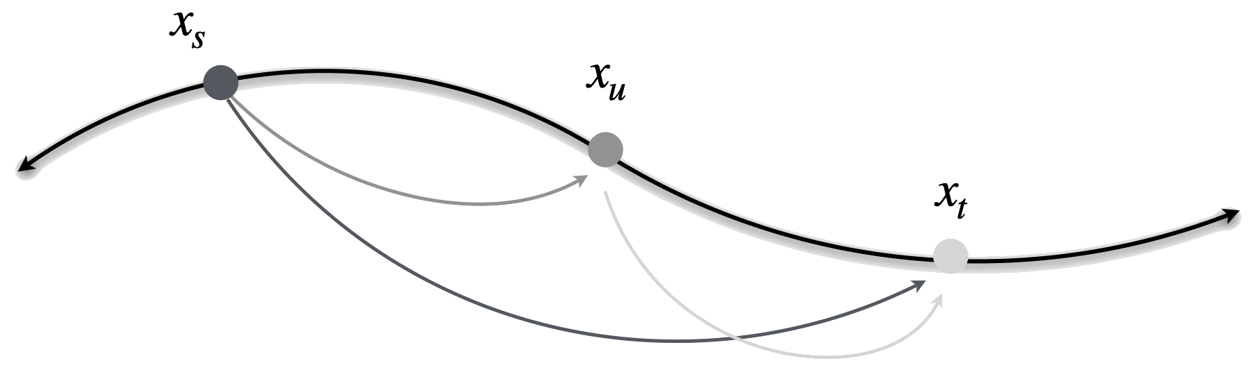
The idea is to learn the flow map $X_{s,t}$, defined as the solution operator of the probability flow ODE. By definition, it satisfies
$$X_{s,t}(\mathbf{x}_s) = \mathbf{x}_t$$for any pair of times $(s, t)$, directly transporting between any two points on the flow without tracing the intermediate path. Unlike discrete diffusions, this object exists because our continuous flow is deterministic, so that the entire trajectory is determined by the initial Gaussian noise sample. You can think of the flow map as a “teleporter” that says exactly where this noise will end up. In particular, one-step generation is simply
$$\hat{\mathbf{x}}_1 = X_{0,1}(\mathbf{x}_0).$$
Continuous flow. The density smoothly sweeps from $\rho_0$ to $\rho_1$, passing through every intermediate state.
Flow map. The flow map “teleports” the density directly between time points, skipping the intermediate states. With a single map $X_{0,1}$, we jump straight from noise to data.
Learning Flow Maps via Distillation
We learn the flow map by distilling the pretrained flow model. The key property we exploit is called the semigroup property, which states that the flow map from $s$ to $t$ can be decomposed as two consecutive maps $s \to u \to t$. This means we can train the flow map to be self-consistent:
$X_{s,t}(x) = X_{u,t}(X_{s,u}(x))$
By enforcing this composition rule during training, the model learns to take larger and larger jumps while maintaining accuracy. Eventually, it can jump from $s{=}0$ all the way to $t{=}1$ in a single step.
The Two-Time Denoiser
We typically parameterize the flow map as
$$X_{s,t}(x) = x + (t-s)\,v_{s,t}(x),$$where $v_{s,t}$ is the average velocity over the interval $[s, t]$. Just as we reparameterized the velocity as a denoiser, we can reparameterize the flow map as a two-time denoiser,
$$\delta_{s,t}(x) = x + (1-s)\,v_{s,t}(x),$$which uses the same average velocity $v_{s,t}$ but takes a single step all the way to $t{=}1$. This object has an important property: it always lies on the probability simplex, regardless of the time interval $(s, t)$. This means we can train it with the cross-entropy loss, inheriting all the benefits of the classification formulation.
When $s = t$, the two-time denoiser reduces to the ordinary denoiser $D_s$. When $t = 1$, $\delta_{s,1}(x) = X_{s,1}(x)$, giving the final prediction directly. Given the two-time denoiser, we can always reconstruct the flow map via
$$X_{s,t}(x) = \frac{1-t}{1-s}\,x + \frac{t-s}{1-s}\,\delta_{s,t}(x).$$That is, the two-time denoiser gives a lossless reparameterization of the flow map that always lives on the simplex, letting us learn the flow map entirely through classification.
Two-time denoiser $\delta_{s,t}$. The two-time denoiser maps a noisy point at time $s$ to a prediction on the simplex, parameterizing the flow map while always remaining on the probability simplex.
Three Distillation Objectives
There are three equivalent mathematical characterizations of the flow map, each giving rise to a different distillation objective. All three characterize the same object, but they construct the teacher signal in fundamentally different ways. We focus on the semigroup objective for our main results, and briefly describe the alternatives for completeness.
Semigroup. The idea behind semigroup distillation is progressive composition. We start from the pretrained velocity field, which can only take infinitesimal steps, and train the model to compose pairs of short jumps into single longer jumps. The teacher signal for a jump from $s$ to $t$ is a convex combination of two shorter jumps through an intermediate time $u$,
$$\bar{\delta}_{s,t} = \gamma\,\hat{\delta}_{s,u}(I_s) + (1{-}\gamma)\,\hat{\delta}_{u,t}(X_{s,u}(I_s)).$$Because the teacher is a convex combination, it always stays on the probability simplex and requires only forward evaluations. Over the course of training, the model learns to make progressively larger jumps, until a single jump from $t{=}0$ to $t{=}1$ produces coherent text.
Semigroup distillation. The teacher is a convex combination of two shorter jumps on the simplex. No derivatives needed, only forward evaluations.
Lagrangian. The Lagrangian approach takes a “follow the particle” perspective. It transports the noisy sample $I_s$ forward along the learned flow to time $t$, evaluates the pretrained denoiser $D_t$ at the transported point, and then applies a correction involving the time derivative $\partial_t \hat{\delta}$ of the student. This derivative requires a Jacobian-vector product to compute, making the objective more expensive than the semigroup alternative. The resulting teacher signal is
$$\bar{\delta}_{s,t} = D_t(X_{s,t}(I_s)) - \tfrac{(1-t)(t-s)}{1-s}\,\partial_t \hat{\delta}_{s,t}(I_s).$$Lagrangian distillation. The teacher is constructed by transporting $I_s$ forward along the flow, applying the pretrained denoiser at the transported point, and correcting with $\partial_t \hat{\delta}$.
Eulerian. The Eulerian approach takes the opposite perspective: instead of transporting the sample, it stays at the starting point and uses derivative information to predict where the flow would go. The teacher evaluates the pretrained denoiser $D_s$ at the initial point $I_s$ and corrects using both a time derivative and the spatial Jacobian of the student. This requires more derivative information than the Lagrangian, but avoids the need to transport the sample forward. The resulting teacher signal is
$$\bar{\delta}_{s,t} = D_s(I_s) + \tfrac{t-s}{1-t}\Big((1{-}s)\,\partial_s \hat{\delta}_{s,t}(I_s) + (D_s(I_s) - I_s) \cdot \nabla \hat{\delta}_{s,t}(I_s)\Big).$$Eulerian distillation. The teacher uses the pretrained denoiser at the starting point, corrected by the Jacobian of the student.
All three objectives also have self-distillation variants (Prop. C.11 in the paper [1]), where the model trains from scratch without a pretrained teacher. The diagonal term becomes standard flow matching (cross-entropy to one-hot data), and the off-diagonal teacher uses the model's own predictions. This connects the Eulerian self-distillation to consistency models and MeanFlow, and the Lagrangian self-distillation to terminal velocity matching. A unified treatment of all three families can be found in How to Build a Consistency Model and Flow Map Matching.
7. Putting It All Together
The full pipeline works in two stages:
Stage 1: Train FLM. We train a flow-based language model using the denoiser parameterization with the cross-entropy loss. A key ingredient is a time reparameterization based on the decoding error rate—the probability that the current noisy state decodes to the wrong token. This redistributes training effort so that each step contributes equally to denoising, which is critical when the vocabulary is large.
Time Reparameterization: Why It Matters
The decoding error rate $P_e(t)$ measures what fraction of tokens are incorrectly decoded at time $t$. For the linear interpolant, $P_e$ stays high for most of the interval and drops sharply only near $t{=}1$—meaning most of the "action" is concentrated in a tiny time window. Uniform time sampling wastes most of the training budget on times where nothing interesting happens.
The reparameterization $\tau(t) = 1 - \frac{|V|}{|V|-1} P_e(t)$ rescales time so that each unit of $\tau$ corresponds to equal progress in resolving tokens. Compare the two animations below: with uniform time, points (colored red when incorrectly decoded, blue when correct) stay red for most of the animation and snap to blue only at the very end. With reparameterized time, the transition is spread evenly, giving the model uniform signal throughout training.
Uniform time. Points stay incorrectly decoded (red) for most of the interval and snap to correct (blue) only near $t{=}1$.
Reparameterized time. In $\tau$-space, each particle turns blue at a regular interval, reflecting uniform denoising progress.
Stage 2: Distill into FMLM. We distill FLM into a flow map language model using the two-time denoiser parameterization. Since both the two-time denoiser $\hat{\delta}_{s,t}$ and the semigroup teacher $\bar{\delta}_{s,t}$ lie on the probability simplex, we can train using a KL-based semigroup objective,
$$\mathcal{L}_{\mathsf{KL}}(\hat{\delta}) = \mathbb{E}_{s,u,t}\,\mathbb{E}_{\mathbf{x}_0, \mathbf{x}_1}\Big[\sum_{l=1}^L \mathsf{KL}\big(\bar{\delta}^l_{s,t} \,\Vert\, \hat{\delta}^l_{s,t}(I_s)\big)\Big] + \mathbb{E}_t\,\mathbb{E}_{\mathbf{x}_0, \mathbf{x}_1}\Big[\sum_{l=1}^L \mathsf{KL}\big(\hat{D}^l_t(I_t) \,\Vert\, \hat{\delta}^l_{t,t}(I_t)\big)\Big],$$where the first term enforces the semigroup condition and the second (diagonal) term ties $\hat{\delta}_{t,t}$ to the pretrained denoiser $\hat{D}_t$. The distilled model can generate text in 1, 2, 4, or 8 steps.
8. Results
We evaluate on two standard benchmarks: LM1B (One Billion Word) and OpenWebText (OWT), measuring generative perplexity (lower is better) and entropy (should match the dataset's entropy).
Many-step generation
At 1024 steps, FLM already outperforms all discrete diffusion baselines, achieving 96.91 generative perplexity on LM1B (vs. 98.14 for the best baseline, Duo [6]) and 62.23 on OWT (vs. 77.69). This shows that continuous flows are not just useful for speedup—they produce better samples even in the many-step regime.
Few-step and one-step generation
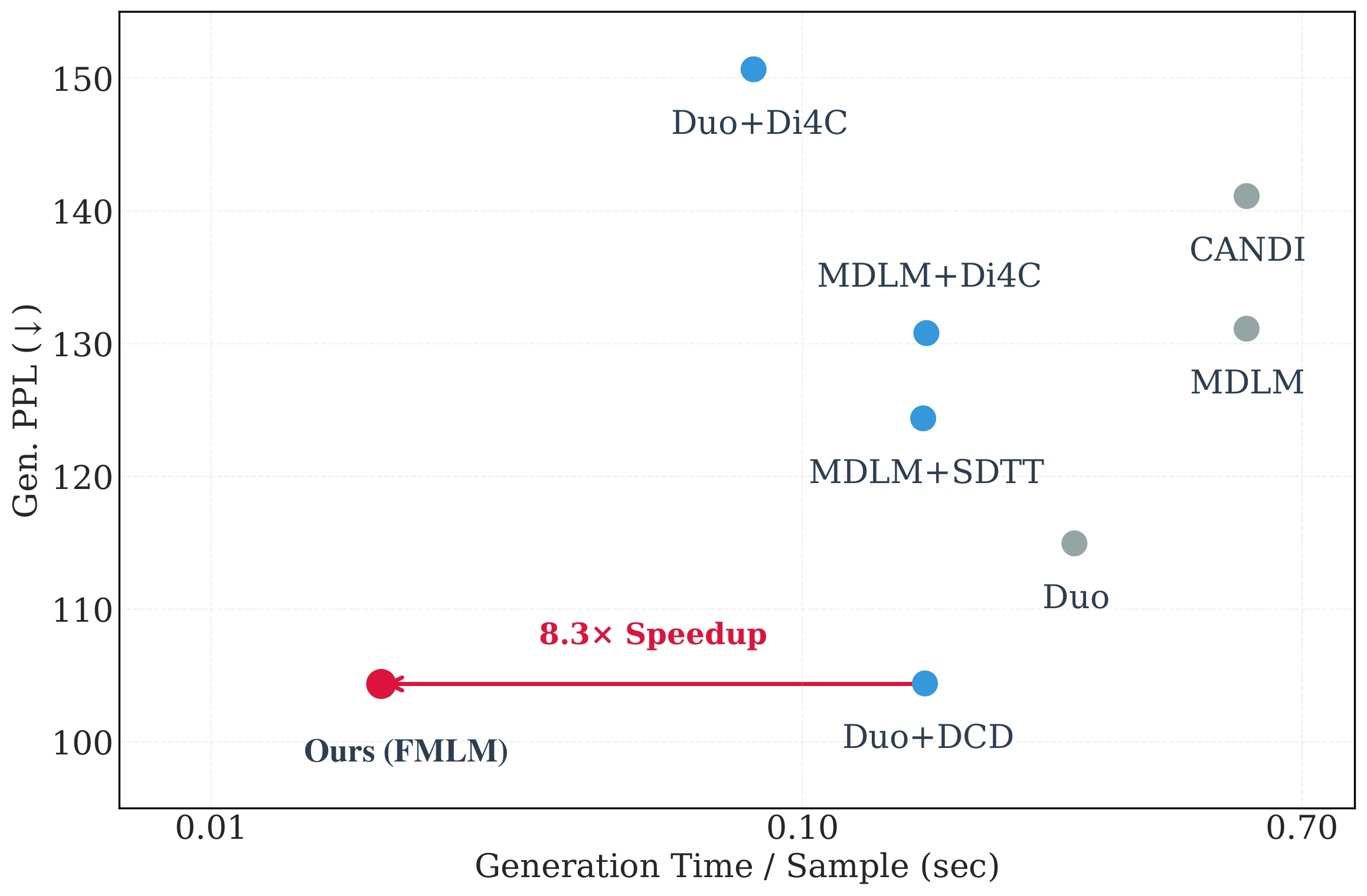
The real story is in the few-step regime, where FMLM dramatically outperforms distilled discrete diffusion:
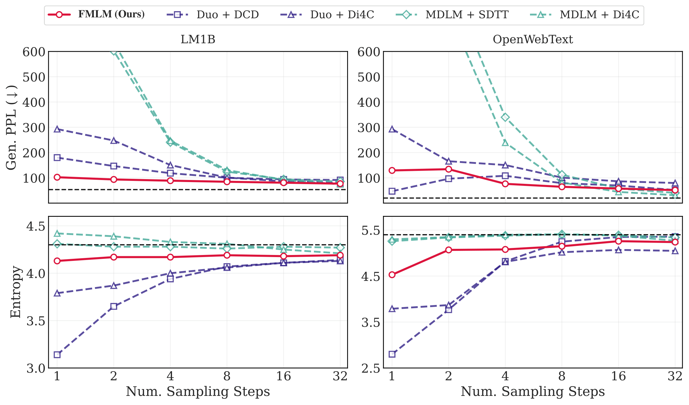
Qualitatively, the difference is even more striking. At one step, discrete diffusion baselines produce either garbled text (generative perplexity >1200) or degenerate text (entropy collapse to 3.79). FMLM generates coherent, grammatically-reasonable sentences while maintaining entropy close to the dataset.
Why does it work?
Our ablation studies validate each of the design decisions underlying FLM and FMLM.
Parameterization matters above all else. Velocity prediction with MSE loss fails to converge (generative perplexity of 3801), confirming the rank bottleneck induced by regressing onto Gaussian noise targets in the high-dimensional one-hot space. The denoiser parameterization with cross-entropy achieves 97, validating our development of the denoiser as a posterior density that exploits the discrete structure of the data.
Time reparameterization is critical for large vocabularies. Our decoding error rate reparameterization outperforms uniform sampling, learned entropic time, and rank-based reparameterization, confirming that concentrating training signal where tokens are actually being resolved is more effective than learning the schedule. Without it, generative perplexity jumps from 107 to 149.
One-hot encodings outperform all embedding alternatives, including learned embeddings with L2 normalization and frozen BERT embeddings. Notably, simplex diffusion (which constrains the flow to the simplex) suffers severe entropy collapse. We hypothesize that this occurs because, in high dimensions, all samples are initialized from the uniform discrete distribution, leading to very little diversity from the initial condition. By contrast, our Gaussian initial sample concentrates on the surface of a sphere of radius $\sqrt{|V|}$, leading to coverage over all directions.
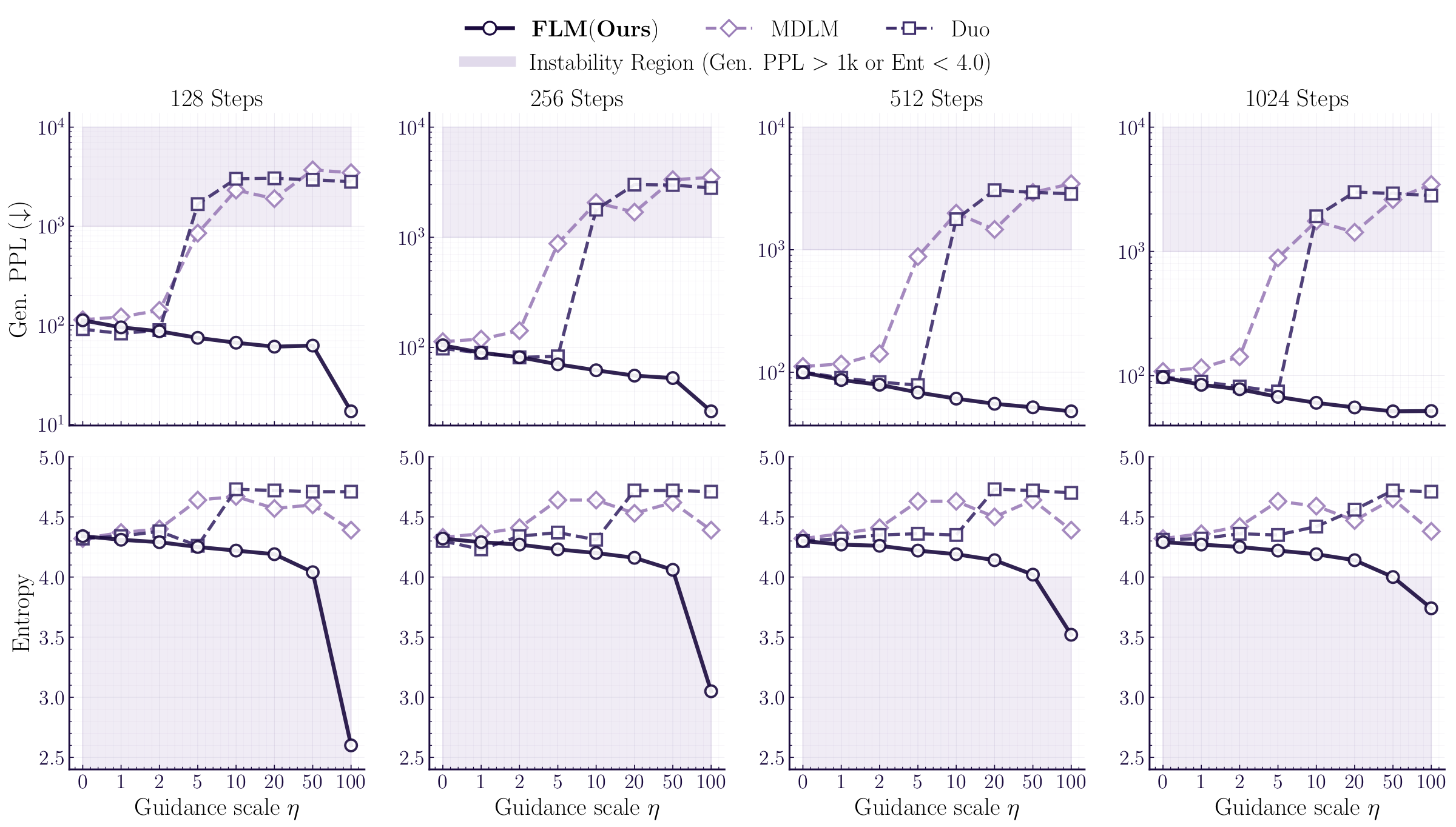
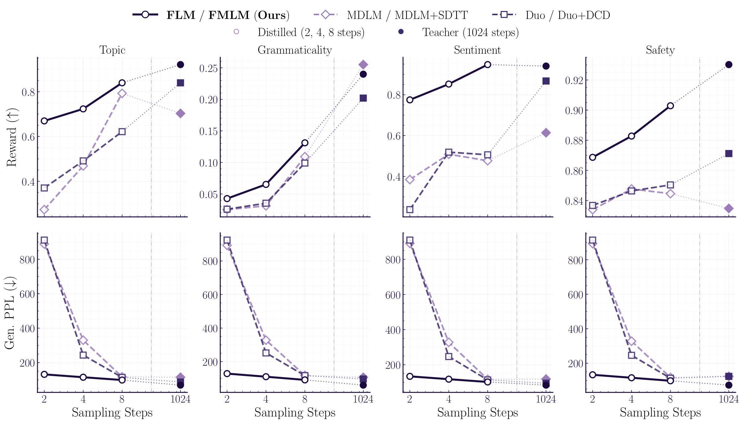
The continuous formulation enables inference-time guidance. Because our flow is deterministic and differentiable, we can apply autoguidance at inference time, or use reward classifiers to steer generation via a differentiable look-ahead that is unavailable to discrete methods.
FLM with autoguidance reaches 51.62 generative perplexity on LM1B, while discrete baselines collapse under the same guidance strength. With reward-guided generation, we can steer toward desired attributes like topic, grammaticality, sentiment, and safety, even at very few steps.
Looking Forward
This work challenges the widely-held assumption that discrete noising processes are necessary for generative modeling over discrete data like text. By showing that continuous flows can outperform discrete diffusion in both quality and speed, we open the door to leveraging the rich toolkit of continuous generative modeling—including guidance, inversion, and editing—for language generation.
We believe the most exciting direction is scaling: our 179M-parameter model already achieves strong results, and the approach is fully compatible with modern transformer architectures. As these models grow, one-step language generation could become a practical alternative to autoregressive decoding.
For the full technical details, see our paper [1]. Code is available on GitHub.
Citation
If you find this work useful, please cite:
@article{lee2026flow,
    title={Flow Map Language Models: One-step Language Modeling via Continuous Denoising},
    author={Chanhyuk Lee and Jaehoon Yoo and Manan Agarwal
            and Sheel Shah and Jerry Huang
            and Aditi Raghunathan and Seunghoon Hong
            and Nicholas M. Boffi and Jinwoo Kim},
    journal={arXiv preprint arXiv:2602.16813},
    year={2026}
}
References
- Lee et al. Flow Map Language Models: One-step Language Modeling via Continuous Denoising. arXiv 2026.
- Albergo, Boffi, Vanden-Eijnden. Stochastic Interpolants: A Unifying Framework for Flows and Diffusions. arXiv 2023.
- Song et al. Consistency Models. ICML 2023.
- Geng et al. Mean Flows for One-step Generative Modeling. NeurIPS 2025.
- Zhou et al. Terminal Velocity Matching. ICLR 2026.
- Boffi et al. Flow Map Matching with Stochastic Interpolants: A Mathematical Framework for Consistency Models. arXiv 2025.
- Boffi, Albergo, Vanden-Eijnden. How to Build a Consistency Model: Learning Flow Maps via Self-Distillation. NeurIPS 2025.
- Sahoo et al. The Diffusion Duality (Duo). ICML 2025.
- Sahoo et al. Simple and Effective Masked Diffusion Language Models (MDLM). NeurIPS 2024.
- Deschenaux et al. Beyond Autoregression: Fast LLMs via Self-Distillation Through Time (SDTT). ICLR 2025.